Compare attenuation and dispersion

What you should be able to do

Distinguish a reduction in optical power from spreading of a pulse in time, and explain why an acceptable loss result does not answer every transmission-performance question.

Attenuation

Attenuation is a reduction in optical signal power between defined points. A loss ratio is expressed in dB. A fiber attenuation coefficient may be expressed in dB/km at a stated wavelength. The total installed link also includes the effects of connections and other relevant components; a per-kilometer fiber value is not the complete channel result.

Dispersion

Dispersion changes the timing distribution of the signal. A pulse can spread in time and interfere with neighboring pulses. The receiver may then have difficulty distinguishing the intended data. This is a different problem from simply receiving too little average optical power.

Read the original diagrams

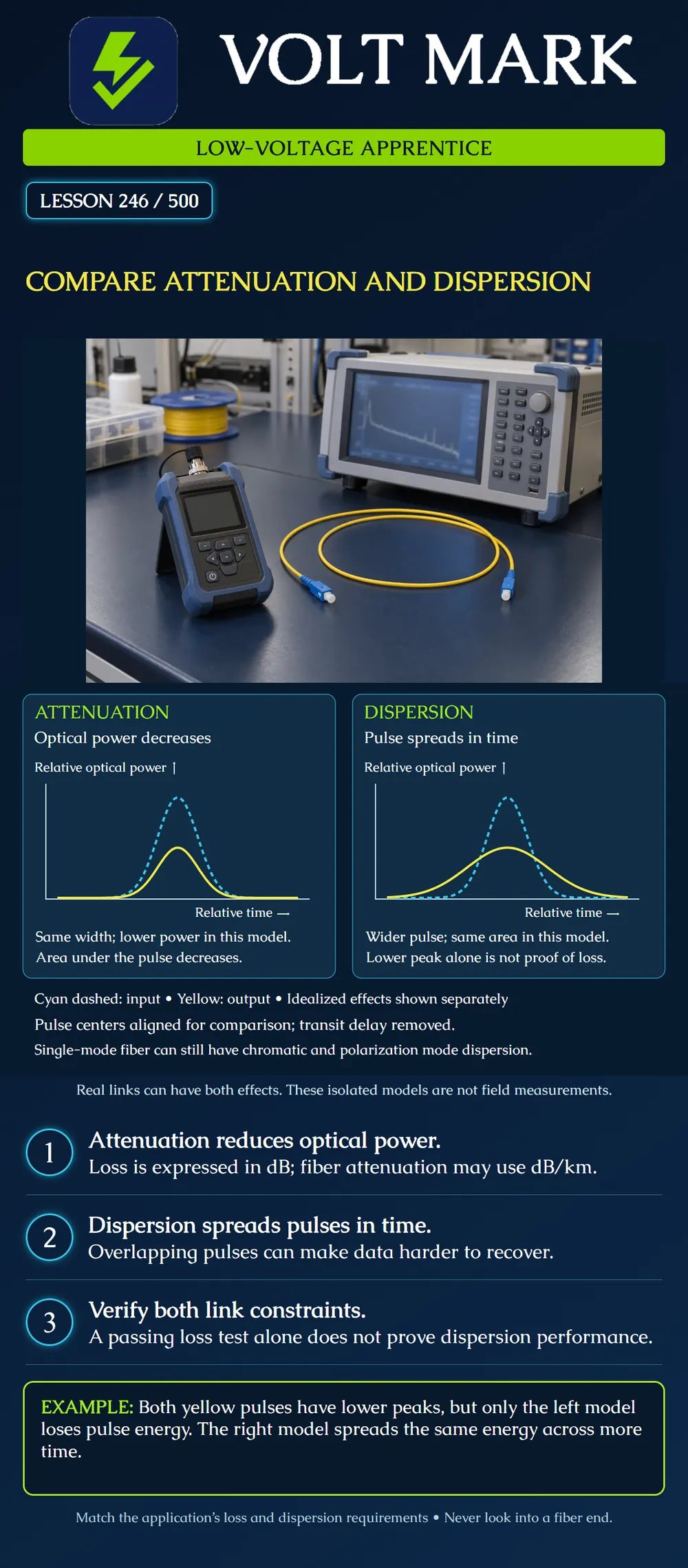
Both plots use relative optical power vertically and relative time horizontally. Cyan dashed lines represent input pulses; yellow lines represent output pulses. Their centers are aligned solely for comparison, with propagation delay removed. They are constructed teaching models, not instrument traces.

Left: an idealized attenuation-only model halves the pulse amplitude without changing its width. The area under the optical-power pulse decreases.

Right: an idealized dispersion-only model doubles the pulse width while halving its peak. For these Gaussian curves, the area is unchanged. The same pulse energy is distributed across a longer time. A lower peak is therefore not, by itself, proof that energy was lost.

Real systems can have attenuation, dispersion and other distortions together. Do not use these sketches as a diagnostic rule that every actual pulse must have a particular shape.

Original model check

For a Gaussian power pulse with peak A and width parameter sigma, area is proportional to A x sigma. Input model: A = 1, sigma = 1; relative area factor = 1. Attenuation-only output: A = 0.5, sigma = 1; relative area factor = 0.5. Dispersion-only output: A = 0.5, sigma = 2; relative area factor = 1.

The factors compare the constructed curves only. They do not specify actual nanoseconds, watts, cable length or an acceptance limit. Pulse energy is the area under power versus time; it is not simply the height of the curve.

Different dispersion mechanisms

Modal dispersion involves different propagation times among modes in multimode fiber. Chromatic dispersion involves wavelength-dependent propagation delay and can affect single-mode links. Polarization mode dispersion involves differential delay associated with polarization states and can also affect single-mode links.

The importance of each depends on fiber, wavelength, transmitter characteristics, data rate and application. “Single-mode” does not mean “no dispersion.” More advanced lessons address measurement units, budgets and long-link assessment; this introductory lesson does not prescribe one universal dispersion threshold.

Original troubleshooting scenario

A link has a recorded passing insertion-loss result, but the data connection does not meet its required performance. An apprentice concludes that the fiber cannot be involved because loss passed.

A better conclusion is narrower: the tested loss condition met its selected criterion. Confirm the application, compatible optics, fiber type, actual route, receiver limits and other required transmission characteristics. A loss pass does not rule out dispersion, a configuration problem or another fault. Likewise, a data error alone does not prove dispersion is the cause.

Choose evidence that answers the question

Original comparison exercise

For each statement, identify what is actually established:

1. “Received average optical power is below the specified minimum.” This identifies a power-level problem requiring investigation; it does not alone identify its cause.
2. “The modeled pulse is twice as wide with the same area.” This demonstrates time spreading without modeled pulse-energy loss.
3. “The cable is single-mode.” This identifies a fiber family; it does not establish that chromatic dispersion or PMD is irrelevant.
4. “The loss report says PASS.” This establishes only the result within that report's verified scope and setup.

Knowledge check

Worked through

Use the lesson's constructed Gaussian model, with the same proportionality constant for all three curves. The input area factor is 1 x 1 = 1. An output peak of 0.5 and width parameter 1 gives 0.5 x 1 = 0.5, so this model retains half the input pulse energy. A second output has the same 0.5 peak but width parameter 2: 0.5 x 2 = 1. Its modeled energy is unchanged while its duration is broader.

The conclusion follows from the area comparison, not the matching output heights. The first is the attenuation-only teaching model and the second the dispersion-only model. An actual trace could include both effects; neither this arithmetic nor a passing insertion-loss report identifies an actual fault cause.

Where beginners go wrong

Sources